From DICOM to sources: the complete pipeline

The nominal run: a DICOM MRI and an EEG go in, a cortical source estimate comes out. We visualise every stage on the sample example subject.

Every figure on this page was produced by the pipeline on the sample subject shipped with the project. Nothing to recompute in order to read the tutorial.

The single call

The whole surface pipeline (SimNIBS FEM route, Windows-native) fits in one call. Each argument maps to a stage detailed below.

from mri2mne.wrapper import reconstruct_sources

result = reconstruct_sources(
    subject="sample",
    output_dir="D:/derivatives",
    dicom_dir="D:/dicom/sample",         # MRI: a DICOM folder
    eeg_file="D:/eeg/sample.edf",        # EEG to localise
    digitization="D:/dig/sample.elc",    # electrode positions
    simnibs_bin_dir="C:/Users/me/SimNIBS-4.5/bin",
    events="find", event_id={"aud_l": 1},
    tmin=-0.2, tmax=0.5, baseline=(None, 0.0),
    inverse_method="dSPM", snr=3.0,
)
print(result.source_estimate_file, result.peak)

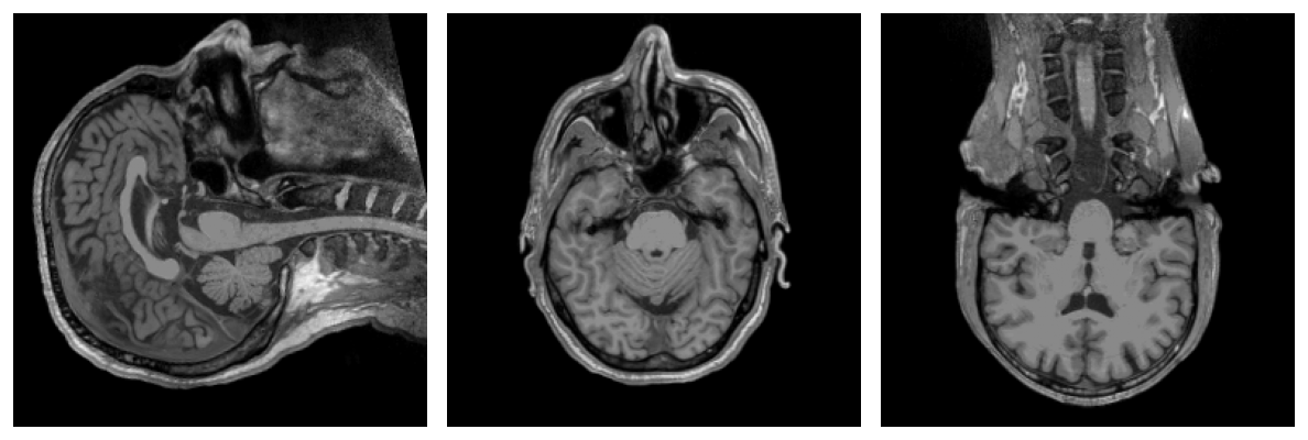
Step 1 — Anatomy (DICOM → T1)

The DICOM folder is anonymised then converted to a single T1 NIfTI volume. That image is all the rest of the pipeline needs.

The <code>sample</code> subject's T1, sagittal, coronal and axial slices. — The `sample` subject's T1, sagittal, coronal and axial slices.

Step 2 — The head model (SimNIBS charm)

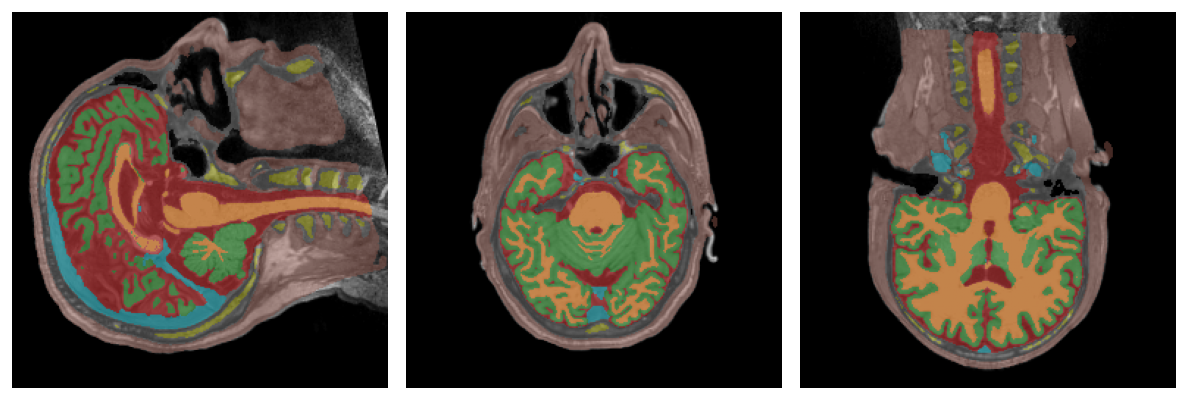
charm segments the T1 into tissues (grey and white matter, CSF, skull, scalp…) and builds a mesh from them. This is the long step (~1–2 h) and the core of the physics: current conduction depends on this anatomy.

Tissue segmentation overlaid on the T1. Each colour is a conductivity class of the FEM model.

Step 3 — Electrodes and EEG signal

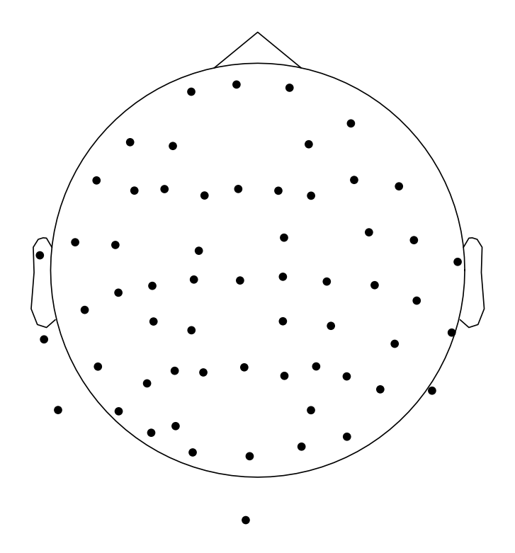
Electrode positions come from the digitisation (EDF stores none). Their labels must match the EEG channels; mismatches are reported, not silently dropped.

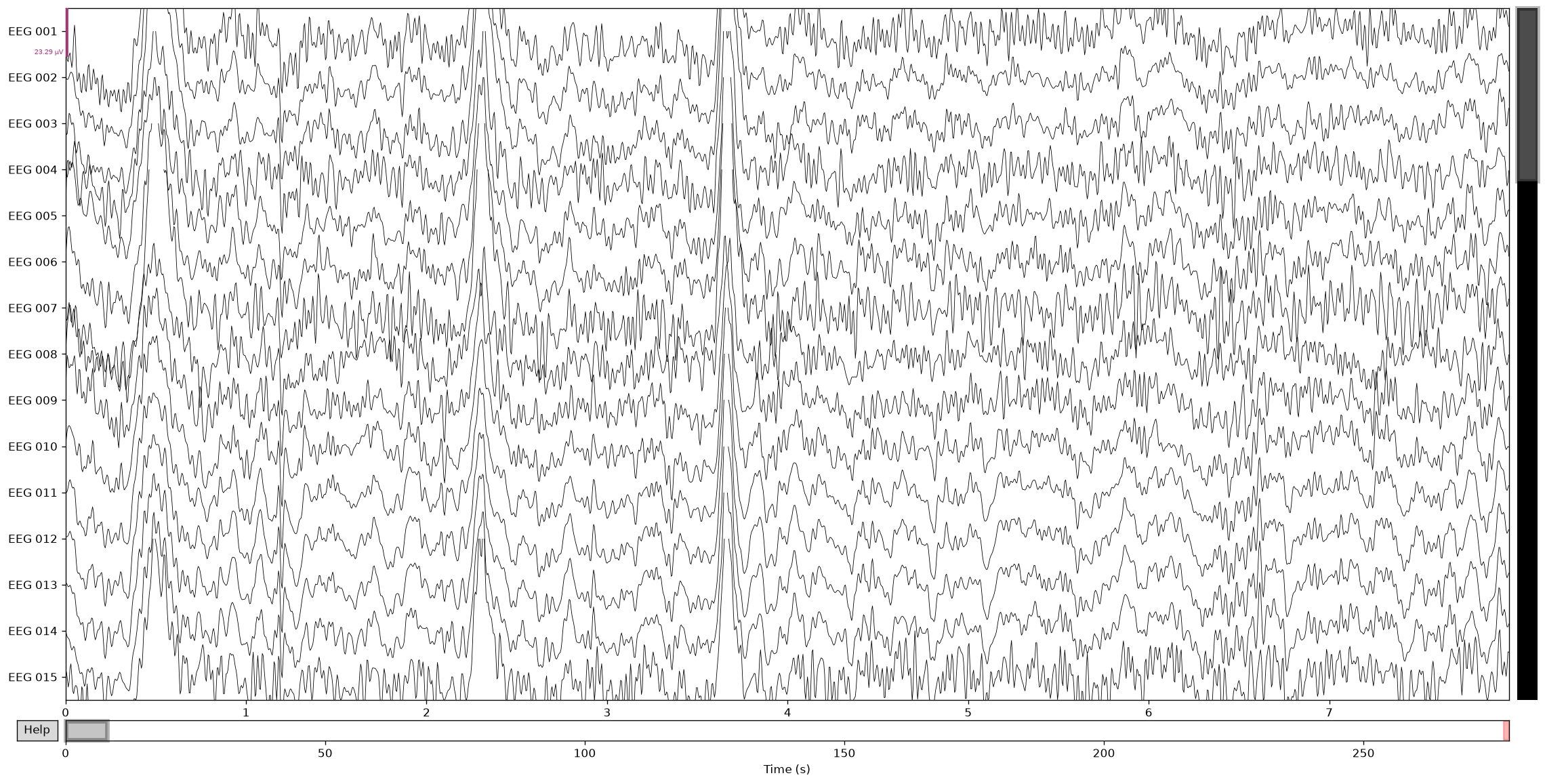
2D layout of the electrodes read from the digitisation.

The continuous recording is read, then band-pass filtered (1–40 Hz by default) and set to an average reference.

A segment of the continuous EEG after filtering.

Step 4 — The evoked response

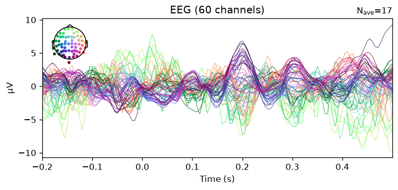
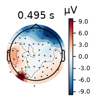
Events cut the signal into epochs, averaged into an evoked response. That is what gets localised. The noise covariance is estimated from the pre-stimulus baseline.

Evoked response, all electrodes overlaid (butterfly plot).

Scalp topography of the potential at the response peak.

Step 5 — Coregistration

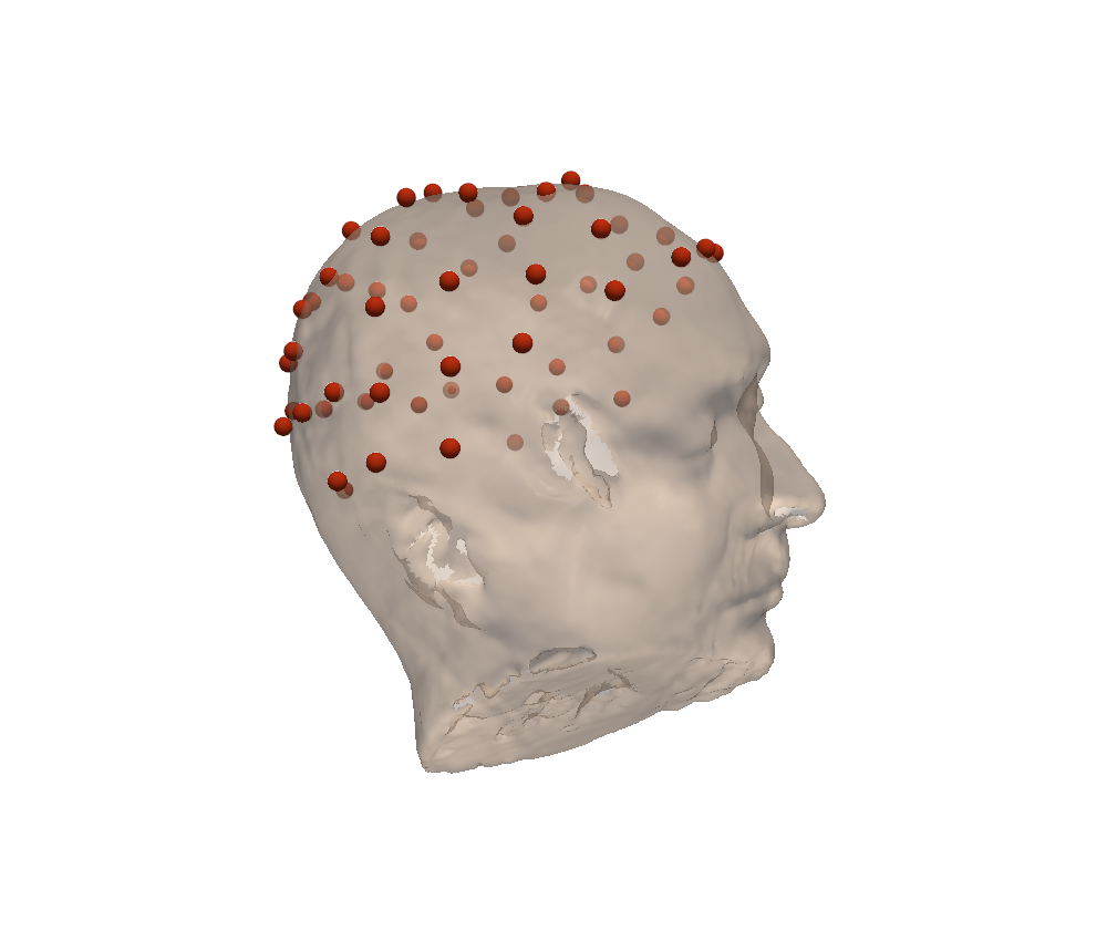
The electrodes are aligned to the mesh-derived scalp (ICP). This is the most sensitive point: a wrong pose shifts the sources without breaking anything downstream, so the residual is measured and plotted for a visual check.

Electrodes (red) sitting on the subject's head surface after coregistration.

Step 6 — The forward model

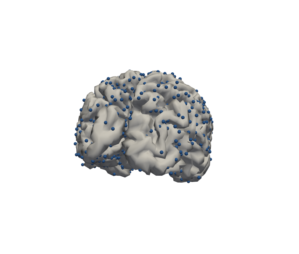
SimNIBS solves the forward problem by finite elements: for each cortical source point, the potential at each electrode. The source space is the central cortical surface.

Source space: points (blue) spread over the cortical surface (one in seven shown).

Step 7 — Inverse and sources

Forward, covariance and EEG combine into an inverse operator (minimum-norm: dSPM here), applied to the evoked response to yield the source estimate on the cortex.

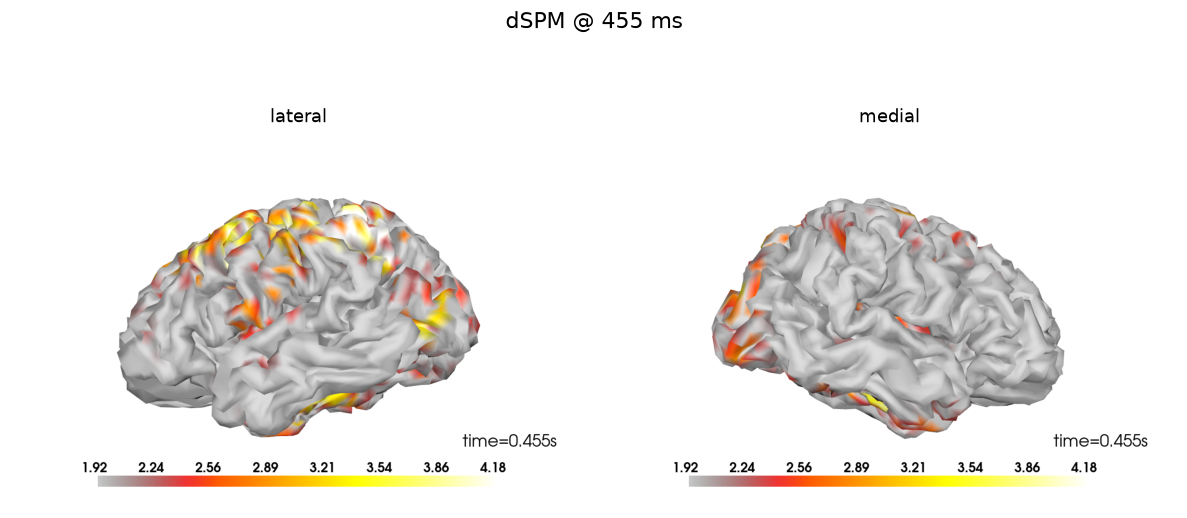
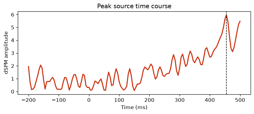
dSPM estimate at the peak, left hemisphere, lateral and medial views.

result.peak gives the location of the maximum in millimetres (MRI frame) and its latency — often the clinical deliverable. A per-subject HTML QC report is written as well.

Where to go next

The scenarios that follow change only a few arguments of this same call: already-preprocessed EEG, an external events file, or starting from a T1 without DICOM.